
該數據集包含來自西班牙的 7500 種不同類型的紅葡萄酒,具有 11 個特徵,描述了它們的價格、評級,甚至一些風味描述,目的為預測價格或品質。[1]
數據包含11個類型:
1. winery: 酒莊名稱
2. wine: 葡萄酒名稱
3. year: 葡萄收穫年分
4. rating: 葡萄酒的平均評分
5. num_reviews: 評論數量。
6. country: 原產地,即西班牙
7. region: 葡萄酒產區
8. price: 價格
9. type: 葡萄酒品種。
10. body: 酒體評分,代表口中葡萄酒的豐富度和重量。
11. acidity: 酸度評分,代表葡萄酒的「皺褶」或酸味。

data在kaggle上Spanish Wine Quality Dataset page上取得。
                        Index: 6070 entries, 0 to 7499
                        Data columns (total 11 columns):
                         #   Column       Non-Null Count  Dtype
                        ---  ------       --------------  -----
                         0   winery       6070 non-null   object
                         1   wine         6070 non-null   object
                         2   year         6070 non-null   int64
                         3   rating       6070 non-null   float64
                         4   num_reviews  6070 non-null   int64
                         5   country      6070 non-null   object
                         6   region       6070 non-null   object
                         7   price        6070 non-null   float64
                         8   type         6070 non-null   object
                         9   body         6070 non-null   float64
                         10  acidity      6070 non-null   float64
                        dtypes: float64(4), int64(2), object(5)
                        memory usage: 569.1+ KB
| winery | wine | year | rating | num_reviews | region | price | type | body | acidity | |
|---|---|---|---|---|---|---|---|---|---|---|
| 0 | Teso La Monja | Tinto | 2013 | 4.9 | 58 | Toro | 995.00 | Toro Red | 5.0 | 3.0 |
| 1 | Artadi | Vina El Pison | 2018 | 4.9 | 31 | Vino de Espana | 313.50 | Tempranillo | 4.0 | 2.0 |
| 2 | Vega Sicilia | Unico | 2009 | 4.8 | 1793 | Ribera del Duero | 324.95 | Ribera Del Duero Red | 5.0 | 3.0 |
| 3 | Vega Sicilia | Unico | 1999 | 4.8 | 1705 | Ribera del Duero | 692.96 | Ribera Del Duero Red | 5.0 | 3.0 |
| 4 | Vega Sicilia | Unico | 1996 | 4.8 | 1309 | Ribera del Duero | 778.06 | Ribera Del Duero Red | 5.0 | 3.0 |
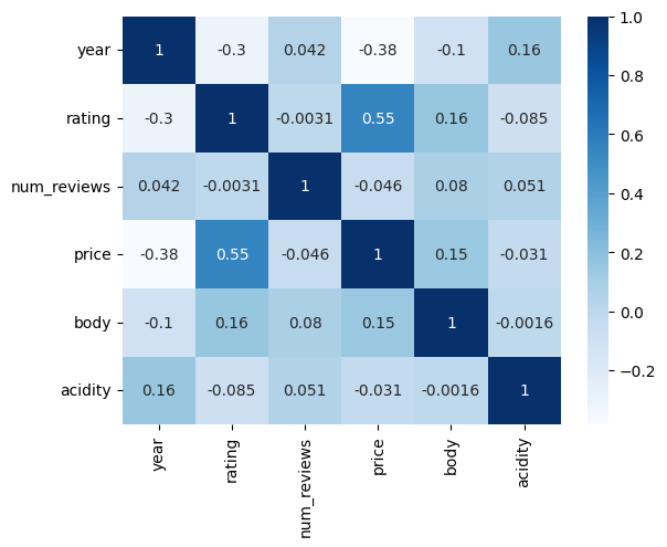
summary: strong relation between price and rating, and specific type of wine will affect price.
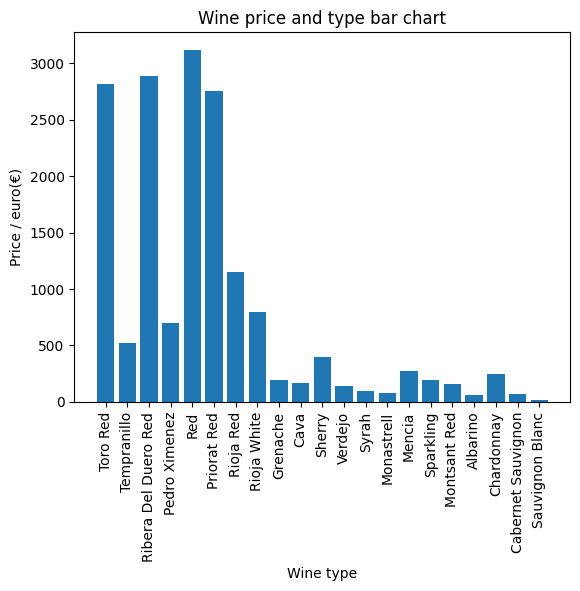
summary: spefic wine have high price, and next step will be finding the model to predict the price.
                        Index: 6070 entries, 0 to 7499
                        Data columns (total 10 columns):
                         #   Column       Non-Null Count  Dtype
                        ---  ------       --------------  -----
                         0   winery       6070 non-null   int32
                         1   wine         6070 non-null   int32
                         2   year         6070 non-null   int64
                         3   rating       6070 non-null   float64
                         4   num_reviews  6070 non-null   int64
                         5   region       6070 non-null   int32
                         6   price        6070 non-null   float64
                         7   type         6070 non-null   int32
                         8   body         6070 non-null   float64
                         9   acidity      6070 non-null   float64
                        dtypes: float64(4), int32(4), int64(2)
                        memory usage: 426.8 KB
                    {'LinearRegression': 0.3997098329164317,
                     'Lasso': -0.0002825894551166108,
                     'Ridge': 0.3997079007354649,
                     'BayesianRidge': 0.3996679858749155,
                     'DecisionTreeRegressor': 0.3963314565148496,
                     'LinearSVR': 0.2089817504376078,
                     'KNeighborsRegressor': 0.5949966180649249,
                     'RandomForestRegressor': 0.7376611282475856}
summary: KNeighborsRegressor and RandomForestRegressor have higher r2 factor, hence we use these two models to generate std price vs. index plots.
                          index  y_prediction  y_actual
                    0      1764     -0.295041 -0.369379
                    1      1821     -0.178520 -0.353428
                    2      1835     -0.256382 -0.348233
                    3      1595     -0.226673 -0.346843
                    4      1731     -0.208753 -0.345574
                    ...     ...           ...       ...
                    1209     42      5.391731  7.383273
                    1210    100      7.117485  7.882926
                    1211    595      3.849200  7.892109
                    1212    199      8.146660  9.494925
                    1213    332      6.879295  9.622104

                    [1214 rows x 3 columns]
                          index  y_prediction   y_actual
                    0      1764     -0.251923  -0.369379
                    1      1947     -0.257671  -0.364968
                    2      1029     -0.267733  -0.359531
                    3      1805     -0.183921  -0.355422
                    4      1821     -0.184619  -0.353428
                    ...     ...           ...        ...
                    1209    595      0.269403   7.892109
                    1210     94     13.041085   7.957844
                    1211     97      4.603715   8.655424
                    1212    188      6.941651  10.383123
                    1213    343      7.828997  16.207611

                    [1214 rows x 3 columns]
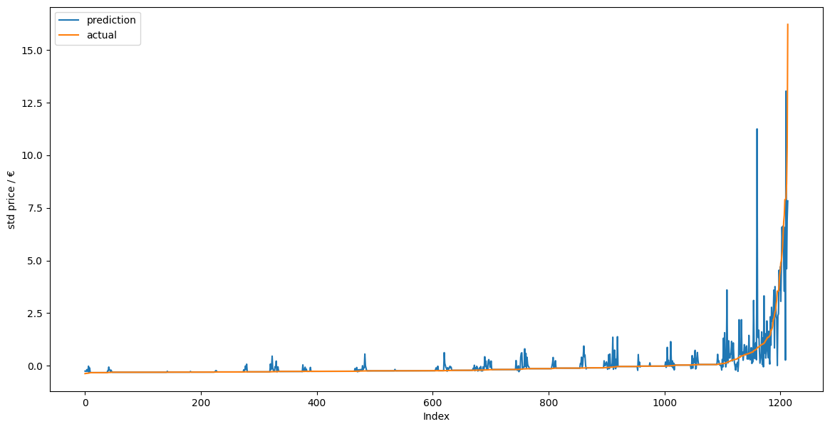
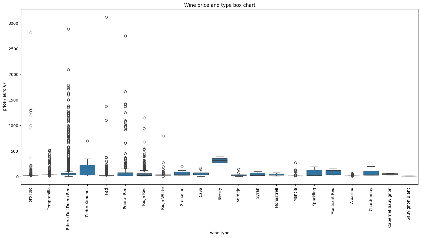
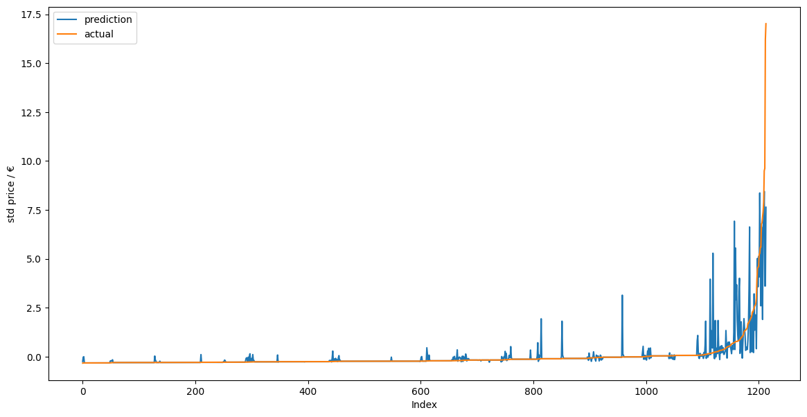
首先經由sort_values(by='y_actual')和reset_index()兩指令使得x軸呈現標準化的low price到high price,y軸則為deviation。可見KNeighborsRegressor model 和 RandomForestRegressor model在index 600下都能有效、正確的預測標準化後的wine price。當index超過800甚至到1000以上時兩model得到的prediction value與actual value相差很大,說明此時model無法預測high price下的actual price。其背後的原因為:從box chart中能發現大部分的wine都屬於low price,當資料量夠大時能得到較準確預測pricce的模型。而high price的wine數量非常少,不容易生成準確的model
因此,我們能用這兩個model來預測特定type的wine的價格(特別在價格不高時)。此練習使用了各式的model,其各自的模型原理還需要再細看。